Analysis

mzML Data Processing

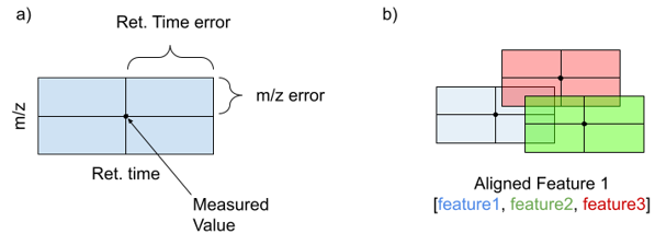
MS features are treated as hyper rectangles where each feature space dimension (ie m/z or retention time) is represented whose edge lengths are determined as the error for the given measurement. The example in two dimensions, m/z and retention time, is given in the figure below (figure part a). However, these rectangles can extend into higher dimensionality as the number of measurements increases. Overlapping rectangles (figure part b) indicate features whose measured values fall within the error of each other, and the mean of all of the measured values are treated as the new Aligned Feature. R-trees are a data structure well suited for the storage and rapid accession of spatial data like the feature rectangles. An R-tree is constructed by calculating user specified error for each feature dimension. In the case of m/z this should be the ppm precision of the instrument on which the data was collected. For retention time and other dimensions, user specified error windows are used. This error is added to and subtracted from each measurement in the input files to create upper and lower bounds (one parallel set of edges of a rectangle). These rectangles are then added to the R-tree and used to query against in future analyses discussed below.

R-tree method for replicate comparison

When experimental replicates are provided, (as defined by a filename convention sample-name_replicate#.mzml) these are first combined using the feature alignment strategy described above. Only features which appear in enough replicates to satisfy a user defined threshold are kept. For instance, if a feature is only detected in 1 out of 3 replicate files (ie no overlapping rectangles are found in other replicates)and the user specifies that it must be present in 2 or more then that feature(s) will not be included in the “replicated” output file.

R-tree method for feature alignment

After replicates have been compared, and features not meeting the threshold have been eliminated, this reduced subset of features is aligned across all files. This process is the same as replicate comparison, except now overlapping features are allowed to be defined from multiple samples. The original origin of replicated features is preserved but resulting aligned features are meant to represent a fingerprint of potentially individual metabolites in the feature space. The resulting features and information about the components that were combined to create these meta features are output to the user.

Activity Score

Definition

Activity Score is a measure of the strength of the phenotype (i.e. how strong and how widespread is the activity).

Calculation

Activity Scores are calculated as the sum of the squares of the average individual bioassay data values for each feature. For example, if a feature is present in three samples the average biological fingerprint for that feature is calculated by averaging the values in each column of the bioassay data. The Activity Score is calculated by summing the squares of each of these values.

Interpretation

Activity Score represents the strength of the biological fingerprint. Therefore, compounds that have strong effects on multiple bioassay features will have high Activity Scores, while compounds that have low activities across all features, or selective strong activities against a small number of features will both have lower Activity Scores.

Selection of Cutoff Values

If the bioassay data has been internally normalized (i.e., contains values in the range (0 to 1) or (-1 to +1) for each column) then the Activity Score values will fall in the range (0 to x) where x is the number of bioassay columns in the bioassay table (i.e. if the bioassay table has 5 columns of values, then the activity score range is 0 - 5).

Importance of Data Normalization

If the bioassay data have not been normalized then the maximum value can be very high, and cutoffs must be modified appropriately. For example, if the bioassay data contains percent inhibition data then the maximum value in a given column is 100, and the sum of the squares of these values can be in the tens of thousands. This is problematic if the bioassay table contains different data types, because a column containing data in the range 0 - 1 will have lower impact on the Activity Score than a column containing percent inhibition values, and the Activity Score will be biased to readouts with larger values.

Cluster Score

Definition

Cluster Score is a measure of the consistency of the activity profile (i.e. how similar are the activity profiles of samples containing the same compound?). CalculationCluster Scores are calculated by averaging the Pearson similarity scores between the bioactivity profiles for all of the samples that an MS feature is in. For example, if an MS feature is in samples A, B, and C then Pearson similarity scores are calculated between the bioactivity profiles of A vs B, A vs C, and B vs C and the average of these three values returned as the Cluster Score.

NOTE: By definition, MS features that appear only once in the sample set will receive a Cluster Score of +1. Typical MS datasets can include large numbers of features that are artefacts of data acquisition. ‘Singleton’ features that are only present in single samples are deprioritized by being manually assigned a Cluster Score of 0. To review singleton features, users can use the Scatter Plot view, setting ‘maximum frequency’ to 1.

Interpretation

Cluster Scores indicate the consistency of a given phenotype, independent of the strength of the biological response. Therefore an MS feature that consistently aligns with a biological fingerprint of 0001000 will yield a higher cluster score than an MS feature that aligns with a biological fingerprint of 1101111 only 50% of the time.

Selection of Cutoff Values

By definition, the minimum Pearson score is -1 (a perfect anti-correlation) and the maximum value is 1 (a perfect correlation). Therefore the range of Cluster scores is always (-1 to +1), regardless of the number of bioassay features or the magnitude of individual values. In our experience setting even a modest positive Cluster Score cutoff (e.g. 0.1) eliminates many MS features from the plots. This improves interpretability and eliminates many inactive features while retaining biologically relevant candidate MS features.

Network Generation

Networks are created in Python using the NetworkX library and exported in the graphML data format.

Node and Edge Creation

Networks are generated by creating nodes for every sample in the bioassay file, and for every MS feature in the MS data that possesses Activity and Cluster Scores above the defined thresholds. Bidirectional edges are then created between each MS feature and the samples it is present in. Therefore, sample nodes are never connected directly by edges, but instead are joined by shared bioactive MS features.

Exclusion of Sample Nodes

Following initial graph creation, sample nodes are removed if they do not possess any edges to MS features in the graph. This can occur when a sample is biologically inactive, and does not contain any MS features that meet the defined score thresholds. Following graph trimming, communities are detected using the Louvain community detection method in NetworkX.

Interpretation

In the network view, samples are grouped together based on shared bioactive features. Therefore, a molecule that generates several different adducts and/or fragments in the mass spectrometer will yield a sub-cluster in the network that is grouped around this set of features. By contrast, a family of related molecules may also create a subcluster in the network, provided that these family members co-occur in the majority of samples within the cluster. Unlike MS-based clustering methods, NP Analyst network groupings are driven by shared bioactive MS features, rather than similarity of MS/MS fragmentation spectra, affording a direct mechanism to prioritize biologically active features.