Covariate projection

Covariates (or confounders) are variables that are associated with both an explanatory and a response variable. In other words, they interfere with or obscure the relationship between the explanatory and response variable. An example is the influence of adiposity (covariate) on the relationship of physical activity (independent variable) and the resulting aerobic fitness (response).

Covariance projection is a method to adjust covariate influence in multivariate datasets by defining a covariance weight vector w_CP that is multiplied with the centered augmented data matrix X_aug that contains X, y and also the covariates z (X_aug = [X, y ,z]). The weight vector w_CP has as many entries as variables exist in X_aug and contains zeros in positions of X and y and ones in z position (= covariate entry). This enables the calculation of the covariance projection scores t_CP and subsequently the loadings p_CP^T.

1) t_CP = X_aug w_CP
2) p_CP^T = t_CP^T X_aug / (t_CP^T t_CP)

Using the loadings and scores, the adjusted augmented E_aug can be calculated (= Dataset after covariate projection in mvpaShiny covariate projection tab).

3) E_aug = X_aug – t_CP p_CP^T

This matrix can be used to perform follow-up analyses like PLS-regression. Ideally, the influence of the covariates have been removed so that the “real” relationship between explanatory and response variables can be determined.

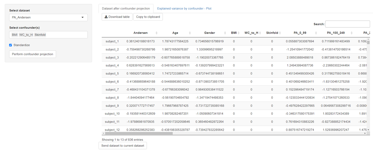
In order to perform the covariance projection in mvpaShiny a dataset needs to be selected (= X_aug) and the covariates have to be defined. Standardization is a useful and recommended step to equalize variables importance. The Perform covariate projection button will start the calculation.

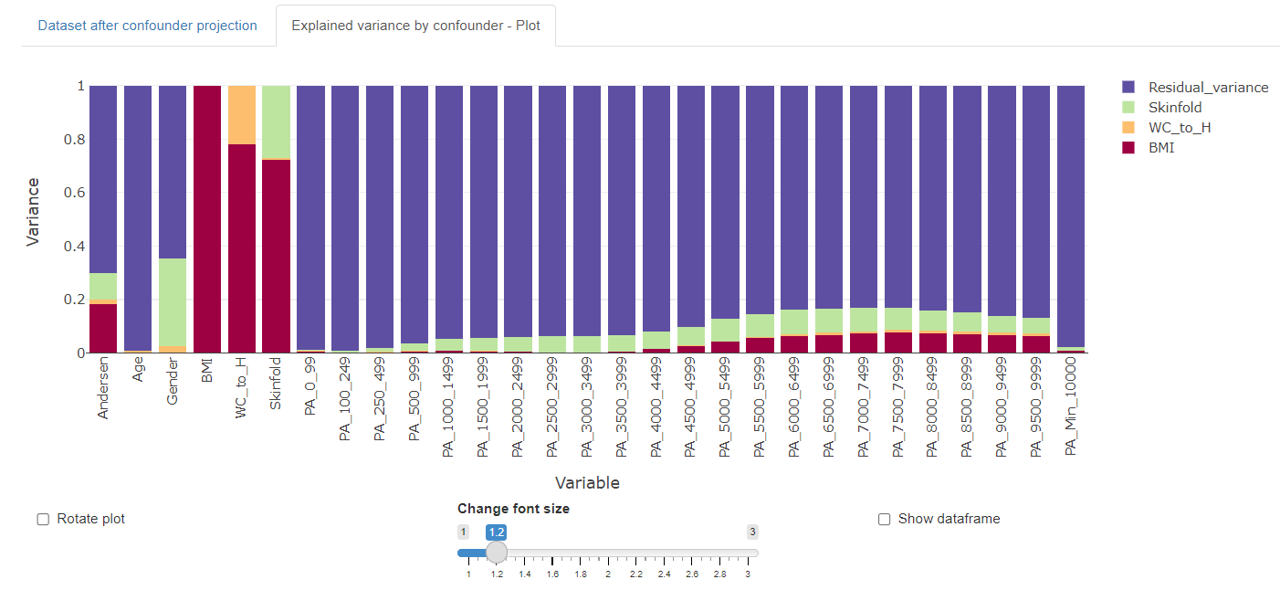
NOTE: The order of selected covariates matters when the explained variance by covariate plot is viewed. While E_aug will be identical, the explained variance by the individual covariate might differ.

Explained variance by covariate plot